Note

Download full notebook here

NIRSpec/G395H Reduction

This notebook will walk you through the basics of data analysis for NIRSpec/G395H BOTS observations. Note that the process to follow will be the same for the other NIRSpec gratings (or PRISM) – we’re using G395H here as an example since that was the mode used in the JWST Transiting Exoplanet Community Early Release Science (ERS) program.

# First thing to do is set your CRDS variables so we can download the most up-to-date JWST
# reference files.

import os
os.environ['CRDS_PATH'] = './crds_cache'
os.environ['CRDS_SERVER_URL'] = 'https://jwst-crds.stsci.edu'

Now let’s get some data! exoTEDRF has a useful functionality which allows you to automatically grab any (public) data from the MAST archive.

Let’s use the WASP-39b transit observations from the JWST Transiting Exoplanet Community Early Release Science program published in Alderson et al. (2023).

from exotedrf.extra_functions import download_observations

# We want all data associated with proposal ID 1366 for target WASP-39b. Additionally we
# specify NIRSPEC/SLIT since this program also observed the same planet with NIRISS and NIRCam.
# Lastly, we want to specify G395H as the filter since this target was also observed with PRISM!

download_observations(proposal_id='1366', objectname='WASP-39b', instrument_name='NIRSPEC/SLIT',
                      filters='G395H')

# This will store all files in a folder in the present directory called DMS_uncal.

Now let’s create output directories to store our data products.

from exotedrf import utils

# Generate output directories
utils.verify_path('pipeline_outputs_directory')
utils.verify_path('pipeline_outputs_directory/Stage1')
utils.verify_path('pipeline_outputs_directory/Stage2')
utils.verify_path('pipeline_outputs_directory/Stage3')
utils.verify_path('pipeline_outputs_directory/Stage4')

exoTEDRF is subdivided into four stages, mirroring the STScI jwst pipeline.

The stages are as follows:

• Stage 1: Detector Level Processing

• Stage 2: Spectroscopic Processing

• Stage 3: 1D Spectral Extraction

• Stage 4: Light Curve Fitting

This notebook will walk you through stages 1 to 3, or from raw data to extracted stellar spectra, mostly following the steps laid out in `Ahrer et al. (2024) <>`__.

Stage 1 – Detector-Level Processing

Stage 1 performs multiple important calibrations on the raw, 4D (integrations, groups, y-pixel, x-pixel) data cubes. Several steps are simply wrappers around the existing functionalities of the STScI pipeline, whose documentation can be found here.

from exotedrf import stage1

# First define some input and output directory paths.

uncal_indir = 'DMS_uncal/'  # Where our uncalibrated files are found.
outdir_s1 = 'pipeline_outputs_directory/Stage1/'  # Where to save our Stage 1 output files.

Now let’s make a list with all the uncal input files. With NIRSpec/G395H, the spectrum is dispersed across two seperate detectors, called NRS1 and NRS2. Each detector has slightly different properties and we will therefore process each of them seperately.

In this case, the full TSO is broken up into three segments for each detector.

filenames_1 = [uncal_indir+'jw01366003001_04101_00001-seg001_nrs1_uncal.fits',
               uncal_indir+'jw01366003001_04101_00001-seg002_nrs1_uncal.fits',
               uncal_indir+'jw01366003001_04101_00001-seg003_nrs1_uncal.fits']

filenames_2 = [uncal_indir+'jw01366003001_04101_00001-seg001_nrs2_uncal.fits',
               uncal_indir+'jw01366003001_04101_00001-seg002_nrs2_uncal.fits',
               uncal_indir+'jw01366003001_04101_00001-seg003_nrs2_uncal.fits']

Let’s check the readout pattern of the observations.

from astropy.io import fits

with fits.open(filenames_1[0]) as file:
    print('No. integrations: {}'.format(file[0].header['NINTS']))
    print('No. groups: {}'.format(file[0].header['NGROUPS']))
    print('subarray: {}'.format(file[0].header['SUBARRAY']))

No. integrations: 465
No. groups: 70
subarray: SUB2048

Here we can see that the full TSO consists of 465 integrations, with 70 groups per integration using the 32x2048 pixel subarray.

Let’s now take a look at what the raw data looks like.

import matplotlib.pyplot as plt

# For NRS1
with fits.open(filenames_1[0]) as file:
    plt.figure(figsize=(8, 3))
    # Let's check out the last group of the 10th integration
    plt.imshow(file[1].data[10, -1], aspect='auto', origin='lower', vmax=3e4)
    plt.text(50, 27, 'Detector NRS1', c='white', fontsize=12)
    plt.show()

# For NRS2
with fits.open(filenames_2[0]) as file:
    plt.figure(figsize=(8, 3))
    # Let's check out the last group of the 10th integration
    plt.imshow(file[1].data[10, -1], aspect='auto', origin='lower', vmax=3e4)
    plt.text(50, 27, 'Detector NRS2', c='white', fontsize=12)
    plt.show()

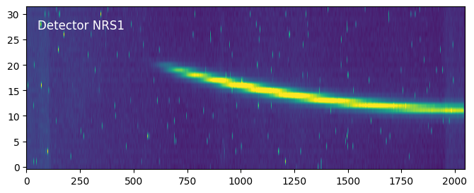
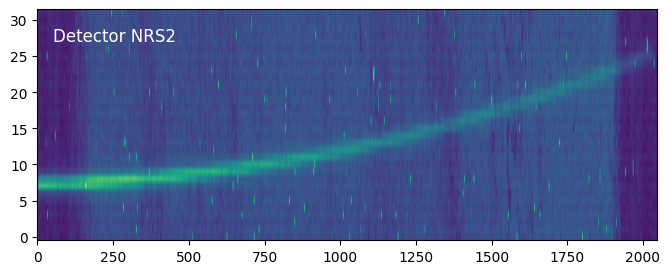
Here we can clearly see the target spectral traces in both detectors as well as a number of detector effects that we need to take care of.

Next, let’s make sure that the observations were successful (i.e., we actually observed a transit).

from exotedrf.plotting import plot_quicklook_lightcurve

# Make a quick a dirty light curve plot.
plot_quicklook_lightcurve(filenames_2)

2025-12-05 08:26:52.943 - exoTEDRF - INFO - Reading file DMS_uncal/jw01366003001_04101_00001-seg001_nrs2_uncal.fits.
2025-12-05 08:26:54.371 - exoTEDRF - INFO - Reading file DMS_uncal/jw01366003001_04101_00001-seg002_nrs2_uncal.fits.
2025-12-05 08:26:55.840 - exoTEDRF - INFO - Reading file DMS_uncal/jw01366003001_04101_00001-seg003_nrs2_uncal.fits.

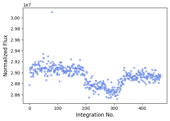
Looks good! The transit is reasonably centered in the time series, and we can already see it clearly even in the raw data! Ingress appears to be around integration 150, and egress at 350. Let’s keep those values in mind to use later.

We’re now ready to start with the actual reduction.

DQ Initalization Step

Intializes the data quality flags and flag saturated pixels.

As mentioned above, NIRSpec/G395H spectra are spread across two detectors, each of which needs to be processed seperately. However, the steps to reduce data from either detector are the same! Any small tweaks required for NRS2 vs NRS1 are automatically handled by exoTEDRF under the hood. Therefore, in order to not repeat every step twice in this tutorial, we’re only going to walk through NRS1 here.

# Initialize the step by passing the input files and the directory to which we want to save
# the outputs.
# There's also an option to pass a custom hot pixel map in order to identify and flag hot pixels
# which are not already in the default data quality map. This should be a boolean map with True
# values for hot pixels and False otherwise. A version of this is output by the BadPixStep towards
# the end of Stage 2.

step = stage1.DQInitStep(filenames_1, hot_pixel_map=None, output_dir=outdir_s1)

# Now run the step!
# This step has options for diagnostic plotting. Specifying do_plot=True will create the step
# plot and save it to the output directory.
# If you want to change the saturation threshold, you can do so by passing a value to the saturation_threshold keyword.
# If not, an instrument-dependent default value will be used.

results = step.run(save_results=True, force_redo=True, do_plot=True)

# Display the step plot.

from IPython.display import Image

Image(filename=outdir_s1 + 'dqinitstep_nrs1.png')

Here we can see a map of all saturated pixels in a frame of the observations — or at least we would if there were any!

Superbias Subtraction Step

Now we subtract the superbias level from all frames.

exoTEDRF offers three ways of determining the bias level for NIRSpec data; two of which are versions of a self-calibration using the first groups of the data itself. The last one uses the standard STScI bias reference file. For simplicitly, that’s the method that we’ll use here.

NOTE: When running the Superbias Correction with the direct outputs of a previous step a specific error may occur: UFuncTypeError: Cannot cast ufunc ‘subtract’ output from dtype(‘float32’) to dtype(‘uint16’) with casting rule ‘same_kind’. This likely stems from a crds reference file compatability issue, and is being looked into. In the mean time, a workaround is to simply create a list of paths to the previous step output files, e.g., results = [‘XXXX_seg001_dqinitstep.fits’, ‘XXXX_seg002_dqinitstep.fits’, …] and pass this to the SuperBiasStep.

# This time we pass the outputs from the previous step as the inputs for this step.
# Passing 'crds' to the method keyword tells the step to use the standard STScI reference file
# instead of a self-calibration.

step = stage1.SuperBiasStep(results, output_dir=outdir_s1, method='crds')

results = step.run(save_results=True, force_redo=True, do_plot=True)

Image(filename=outdir_s1 + 'superbiasstep_1_nrs1.png')

Nine random frames are shown in the diagnostic plot, where we can verify that many of the detector effects we saw above are now gone.

Depending on the superbias subtraction method, other diagnostic plots may be made as well.

Dark Current Subtraction Step

Another wrapper around an STScI pipeline step. This one is optional, and many analyses skip it as the existing dark current reference files show clear residual 1/f noise. Moreover, particularly for NIR observations, the actual dark current signal is extremely small. However, I include it here for completeness!

step = stage1.DarkCurrentStep(results, output_dir=outdir_s1)

results = step.run(save_results=True, force_redo=True)

1/f Noise Correction Step

1/f noise is time-correlated noise which manifests in NIRSpec observations as column-correlated “stripes”. The 1/f noise is actually caused by time-varying voltage levels as the detector is read, and as such it is actually one of the very last noise sources (along with read noise) to be injected into the data. exoTEDRF, therefore, corrects 1/f noise at the group-level (i.e., before ramp fitting).

The 1/f correction also doubles as the background subtraction for NIRSpec/G395H. There are sufficient amounts of non-illuminated pixels in each column to use to estimate both the time-correlated 1/f noise, as well as the faint zodi background signal.

Another thing to note is that although we’re performing this correction now, at the group level, we’re going to repeat it again after ramp fitting. This is just to make extra sure that we’ve removed all the background light and 1/f noise that we can.

For NIRSpec, exoTEDRF provides two different 1/f correction methods. Here, we’re going to use the simplest one, “median”, which simply consists of constructing a median stack for the observation, and subtracting a median of all unilluminated pixels in each column.

It’s a good idea to disclude any bad pixels from the calculation so that we don’t bias the 1/f value calculated for a given column. To address this, there is an optional pixel_masks keyword to which can be passed masks of pixels to exclude in each frame.

If no such masks are available, the step will automatically mask all pixels with non-zero DQ flags, as well as obvious outliers.

pixel_masks = None

# Pixel masks should be boolean arrays (False for "good" pixels and True for pixels to be masked.
# You can either pass one 2D (dimy, dimx) or a series of 3D (nint, dimy, dimx) masks here.

# Initialize the step passing the input files as well as any auxiliary files mentioned above.
# Moreover, we also want to indicate the indices of the baseline integrations and the 1/f
# correction method that we wish to use.

step = stage1.OneOverFStep(results, baseline_ints=[150, -100], output_dir=outdir_s1,
                           pixel_masks=pixel_masks, method='median')

# even_odd_rows=True calculates seperate 1/f noise values for even- and odd-values rows.
# nirspec_mask_width=16 defines the width of pixels around the target spectral trace to mask.
# It's a good idea to make this at least as large as your planned extraction aperture.

results = step.run(save_results=True, even_odd_rows=True, force_redo=True, do_plot=True,
                   nirspec_mask_width=16)

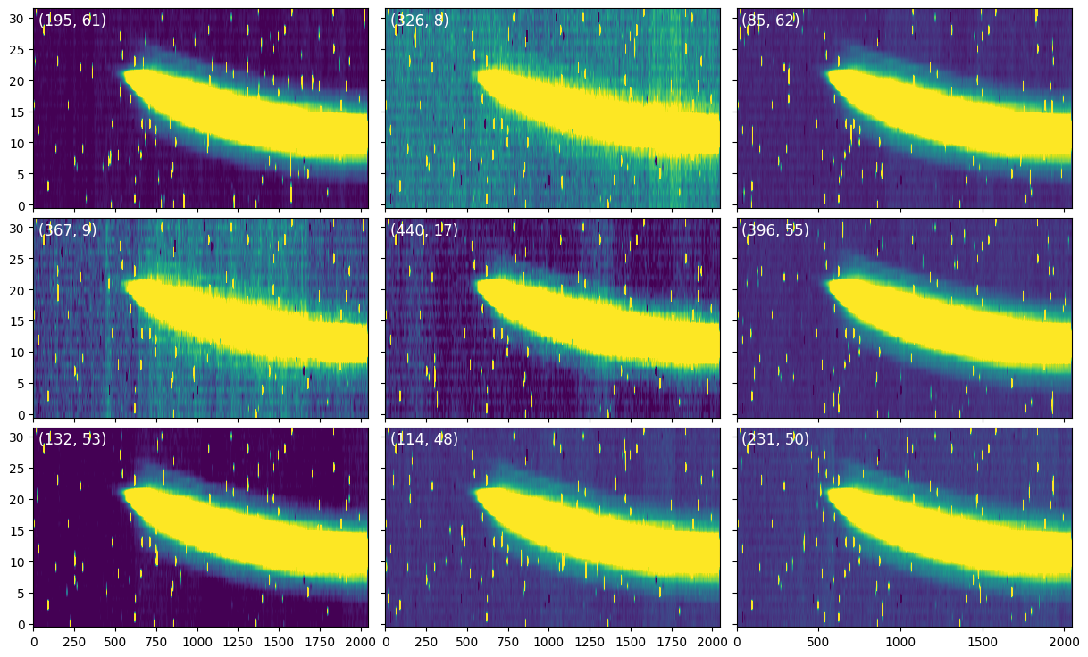
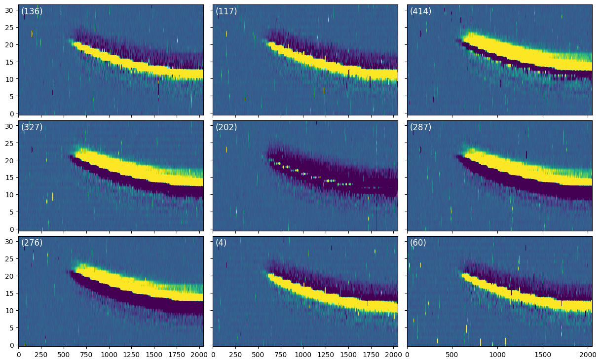
Two diagnostic plots are produced here. The first will be our familiar nine-panel plot, now showing difference images after the 1/f noise correction. We don’t want to see any column-correlated noise left here!

Image(filename=outdir_s1 + 'oneoverfstep_1_nrs1.png')

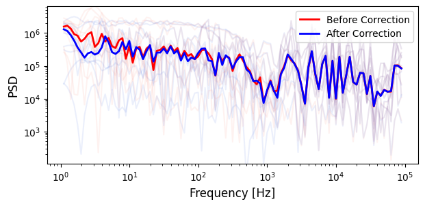
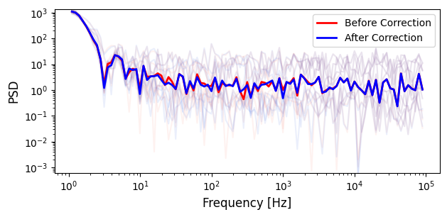
The second is a power series of the data before and after the 1/f correction. The power spectral density before the correction clearly increases, roughly linearly, towards shorter frequencies (hence 1/f!). After the correction though, we can see that the psd is flatter, so we have done a pretty good job of removing all the 1/f noise!

Image(filename=outdir_s1 + 'oneoverfstep_2_nrs1.png')

Linearity Step

The HgCdTe detectors used in NIRSpec are not perfectly linear, which means that as saturation is approached, the counts begin to plateau and less flux is recorded than is actually observed. This is not an issue just with NIRSpec, but all other JWST instruments as well. This step applies pre-calcuated polynomials to correct these non-linearity effects in the ramp.

step = stage1.LinearityStep(results, output_dir=outdir_s1)

results = step.run(save_results=True, force_redo=True, do_plot=True)

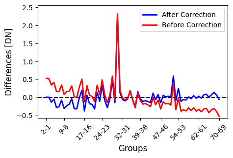
The first diagnostic plot shows (mean-subtracted) group-to-group differences. For a perfect non-linearity correction, we would expect each difference to be identical. The correction is therefore not perfect, but it’s at least a little better than when we started!

Image(filename=outdir_s1 + 'linearitystep_1_nrs1.png')

Jump Detection Step

We now want to detect and flag cosmic ray hits in the data. There are two main ways to do this: up-the-ramp or time-domain flagging.

The up-the-ramp flagging algorithm is the default algorithm in the STScI pipeline. In entails identifying discontinuities above a certain threshold in ramps, and flagging these as jumps. Unfortunately, this method can be quite temperamental and has been found by many studies to flag random noise. It also cannot be applied to ngroup=2 datasets.

The time-domain flagging method uses a sigma clipping algorithm to identify cosmic ray hits in the time domain. This method also has the benefit of working for observations with any number of groups.

step = stage1.JumpStep(results, output_dir=outdir_s1)

# Here we will use the time-domain rejection by specifying flag_in_time=True, and use a clipping
# threshold of 7 sigma.
# In order to use the up-the-ramp flagging, specify instead flag_up_ramp=True and pass an
# appropriate value to the rejection_threshold keyword.

results = step.run(save_results=True, force_redo=True, flag_in_time=True,
                   time_rejection_threshold=7, do_plot=True)

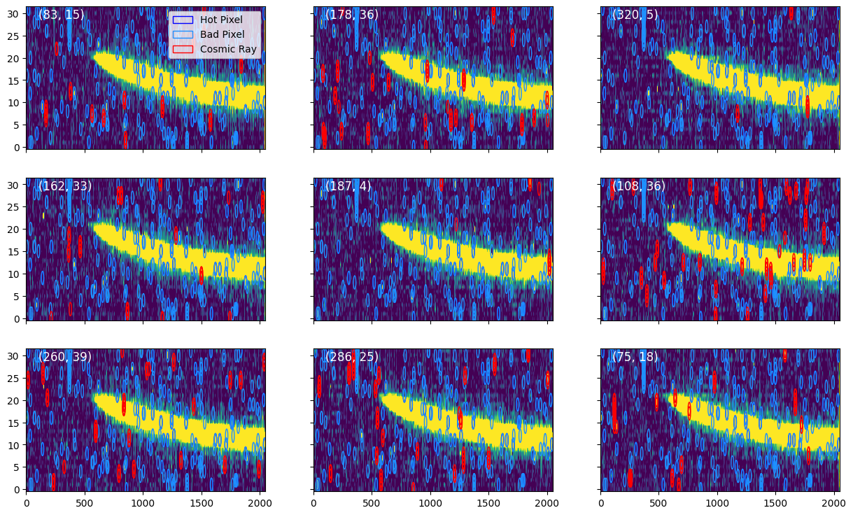
The diagnostic plot here shows the locations of flagged jumps, as well as hot pixels in nine frames.

Image(filename=outdir_s1 + 'jump_nrs1.png')

Ramp Fit Step

Now that all the initial detector-level calibrations are done, we are ready for ramp fitting! This step is a wrapper around the STScI pipeline step that fits a slope and intercept as a function of group to each pixel. We don’t use the intercept values, and only care about the slopes moving forwards.

step = stage1.RampFitStep(results, output_dir=outdir_s1)

results = step.run(save_results=True, force_redo=True)

Gain Scale Step

The gain scale correction does the conversion from DN/s to e-/s by multiplying the data values by the wavelength dependent NIRSpec gain (1.6 e-/DN on average). This is something that can be skipping in many cases, as it won’t affect relative measurements (i.e., transit spectra). However, it is critical if you care about producing flux calibrated products!

step = stage1.GainScaleStep(results, output_dir=outdir_s1)

results = step.run(save_results=True, force_redo=True)

We are now ready to start with Stage 2!

Stage 2 – Spectroscopic Processing

This stage performs some additional calibrations on the, now 3D (integrations, y-pixel, x-pixel), data after the ramp fitting to make the data ready for the spectral extraction. Once again, information on the default STScI pipeline steps can be found here.

from exotedrf import stage2

# Let's now save outputs to the Stage 2 subdirectory.

outdir_s2 = 'pipeline_outputs_directory/Stage2/'

For those of you who have worked through the NIRISS/SOSS tutorial, most of what we’ve done so far will be wuite familiar. However, now we will start to diverge more from that tutorial. This is because unlike NIRISS/SOSS, NIRSpec is a slit spectrograph. Therefore the exact wavelength solution will depend on the positioning of the source within the slit. The next four steps are all mostly wrappers around STScI pipeline steps, with some minor modifications, to derive the wavelength solution of the particular TSO being analyzed.

Assign WCS Step

This is mostly a wrapper around the STScI pipeline step which assigns the appropriate WCS to the data.

step = stage2.AssignWCSStep(results, output_dir=outdir_s2)

results = step.run(save_results=True, force_redo=True)

2D Extraction Step

Here, we use the previously defined WCS in order to create the intial wavelength solution for both detectors. We will then refine this wavelength solution later.

step = stage2.Extract2DStep(results, output_dir=outdir_s2)

results = step.run(save_results=True, force_redo=True)

Source Type Determination Step

For multiple subsequent steps to function, we need to correctly identify the source type in our observations. For all exoplanet TSOs, the correct type is a point source.

step = stage2.SourceTypeStep(results, output_dir=outdir_s2)

results = step.run(save_results=True, force_redo=True)

Wavelength Correction Step

Now that we have defined the precise WCS and know the source type and location within the slit, this step corrects the wavelengths solution in cases where the target is not centered perfectly within the slit.

step = stage2.WaveCorrStep(results, output_dir=outdir_s2)

results = step.run(save_results=True, force_redo=True)

Integration-Level 1/f Correction Step

As mentioned previously, we will now repeat the 1/f and background correction that we did at the group level in order to remove any residual noise that may have managed to slip through.

For all parameters we will use the same inputs as for the group-level correction.

step = stage1.OneOverFStep(results, baseline_ints=[150, -100], output_dir=outdir_s2,
                           pixel_masks=None, method='median')

results = step.run(save_results=True, even_odd_rows=True, force_redo=True, do_plot=True,
                   nirspec_mask_width=16)

Image(filename=outdir_s2 + 'oneoverfstep_1_nrs1.png')

Image(filename=outdir_s2 + 'oneoverfstep_2_nrs1.png')

Inspecting the two plots we can see that not much has changed. Particularly the fact that the power spectrum was already flat even before this second correction shows that we already did an excellent job removing the 1/f noise at the group level. But it’s always good to make sure just in case!

Bad Pixel Correction Step

We are now going to interpolate any remaining bad pixels in the data to be ready for the spectral extraction.

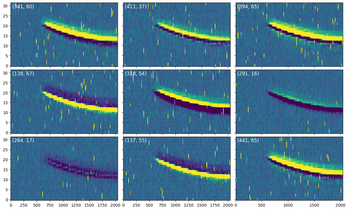
The BadPixStep performs two iterations of bad pixel detection and correction: the first is a spatial correction, and the second a temporal one.

The spatial correction uses a median stack of all integrations to identify any pixels which are systematic outliers across the entire time series. These pixels are flagged, and then interpolate using a median of the surrounding pixels in each integration. Any pixels with DQ flags are also interpolated in this way. It will also produce and save a map of these hot pixels which are not already in the default DQ flags.

The temporal flagging works the same way as the time-domain jump detection, by flagging any pixels which are outliers along the time axis, and replacing them with a median of the surrounding pixels in time.

step = stage2.BadPixStep(results, baseline_ints=[150, -100], output_dir=outdir_s2)

# We're going to use a 10 sigma threshold for both the spatial and temporal corrections.

results = step.run(save_results=True, force_redo=True, do_plot=True,
                   space_thresh=10, time_thresh=10)

Image(filename=outdir_s2 + 'badpixstep_nrs1.png')

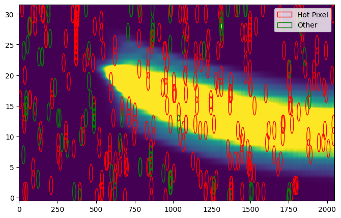
The diagnostic plot here shows the deep stack (median stack) with the locations of all hot and other flagged pixels.

PCA Reconstruction Step

This is the final step of Stage 2. The PCAReconstructStep uses principle component analysis (PCA) to deconstruct the timeseries into eigenimages that explain the largest amount of variance in the data, and their corresponding eigenvector timeseries. We then have the option to reconstruct the data, removing the components which correspond to detector “noise” (e.g., trace position drifts, tilt events, etc.).

step = stage2.PCAReconstructStep(results, baseline_ints=[150, -100], output_dir=outdir_s2)

# We're going to show the first 10 PCA components.

results, deepframe = step.run(save_results=True, force_redo=True, do_plot=True, pca_components=10,
                              remove_components=None)

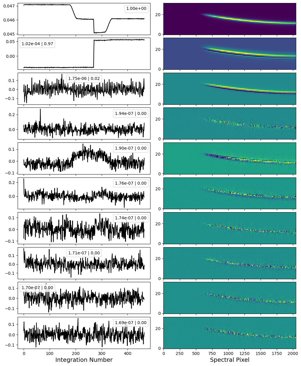
The first diagnostic plot is the intial results of the PCA. Here we see the eigenimages (right) and eigenvalue timeseries (left) of the 10 components that explain the most variance in the data.

The first component is the transit white light curve itself. The second is a so-called “tilt event”, which were more common in the early days of JWST observations. You can actually see that some of the tilt event was picked up by the first component as well.

Beyond that, there is nothing really in these components that are clearly detector noise. So we’re not going to remove anything from the cube.

Image(filename=outdir_s2 + 'stability_pca_nrs1.png')

A good plan of attack is to run this step first, passing remove_components=None to see the initial results. In this case, the step will simply return the input data with no reconstruction. You can then re-run the step specifying the components that you identified as detector-related noise and want to remove.

There is also a nice systematic analysis of NIRSpec/G395H PCA outputs in Gordon et al. (2025) which can help provide some physical insight into the meaning of various eigenimages.

WARNING: Its important to be careful with the number of components being removed. Just like with high resolution cross correlation spectroscopy, removing components can have an effect on the final atmosphere spectrum. Only remove things that you know are detector correlated (positional drifts, beating patterns, etc.). If in doubt, compare your level of light curve scatter as well as the end atmosphere spectrum itself with and without the PCA removal.

Everything looks good! We’re now ready for Stage 3 and the spectral extraction.

Stage 3 – 1D Spectral Extraction

This is the shortest stage, as it just performs the 1D spectral extraction.

from exotedrf import stage3

# Let's now save outputs to the Stage 3 subdirectory.

outdir_s3 = 'pipeline_outputs_directory/Stage3/'

For NIRSpec observations, exoTEDRF can perform a simple box aperture extraction or optimal extraction. For simplicity, we’re just going to use the aperture extraction here.

The Extract1DStep also will locate the positions of the stellar spectral trace on the detector using the the edgetrigger algorithm which was specifically deisgned to handle curved traces as well as overlapping spectral orders (if applicable). The trace centroids will be saved as XXX_nrsX_centroids.csv. For this to work, we also need to pass the deepframe that we created earlier.

step = stage3.Extract1DStep(results, extract_method='box', output_dir=outdir_s3)

# Here, we're using an aperture width of 8 pixels.
# We also pass the deep framne from above.
# Note that if, for whatever reason, you want to specify your own trace positions, you can pass a custom
# centroids file to the centroids keyword.

results = step.run(extract_width=8, deepframe=deepframe, save_results=True, force_redo=True, do_plot=True)

Depending on the extraction method, at least one plot will be made showing the location of the extraction aperture used. Let’s look at that now.

Image(filename=outdir_s3 + 'centroiding_nrs1.png')

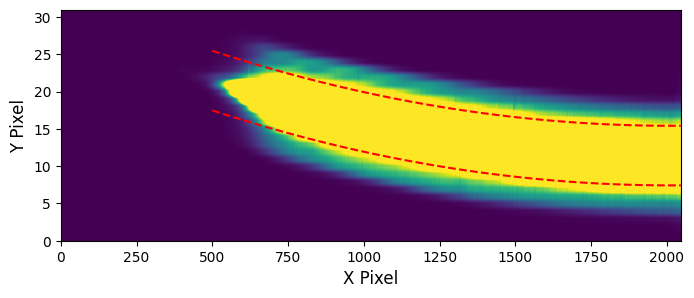
Tada! You now have stellar spectra of WASP-39! Let’s take a quick look at the wavelength-dependent light curves.

For completeness, we’re also going to look at NRS2 at the same time. The NRS2 spectra aren’t directly produced by this notebook since we only ran NRS1. But remember that you can just repeat the same steps as above for NRS2.

import numpy as np

# Open the extracted spectrum file and get the relevant quantities.

with fits.open(outdir_s3 + 'WASP-39_nrs1_box_spectra_fullres.fits') as spec:

    wave_nrs1 = spec[1].data  # NRS 1 wavelengths
    spec_nrs1 = spec[3].data  # NRS 1 spectra

# Do the same for NRS2

with fits.open(outdir_s3 + 'WASP-39_nrs2_box_spectra_fullres.fits') as spec:

    wave_nrs2 = spec[1].data  # NRS 2 wavelengths
    spec_nrs2 = spec[3].data  # NRS 2 spectra

base = np.arange(150).astype(int)  # Baseline integrations

# Normalize the extracted spectra.

spec_nrs1_norm = spec_nrs1 / np.nanmedian(spec_nrs1[base], axis=0)
spec_nrs2_norm = spec_nrs2 / np.nanmedian(spec_nrs2[base], axis=0)

from exotedrf.plotting import make_2d_lightcurve_plot

# For NRS1, only the wavelengths >3µm are useable.

ii = np.where(wave_nrs1 >= 2.9)[0]

# Display the light curves.

kwargs = {'vmin': 0.9725, 'vmax': 1.01}
make_2d_lightcurve_plot(wave_nrs1[ii], spec_nrs1_norm[:, ii], wave_nrs2, spec_nrs2_norm,
                        instrument='NIRSPEC', **kwargs)

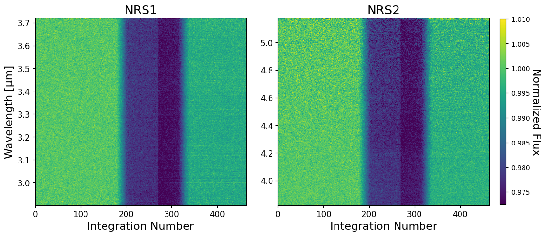
Look at how clean those are!

You’re probably wondering why the second half of the transit is so much deeper than the first. That’s the tilt event that we saw in the PCA earlier! Luckily, it can be easily modelled out using a simple step function.

exoTEDRF Stages 1 to 3 can also be run in script form via the provided run_DMS.py file. Simply fill out the corresponding yaml file with all relevant inputs, and you’re good to go! Generally, I like to take a first pass at the data in a notebook, where I can double check the outputs of each step, and perhaps dig a bit deeper into some interesting things that pop up. I’ll then use the script for the second pass.

You’re now ready to fit some light curves and get your atmosphere spectrum, which is what you really want in the end, isn’t it?!